Citation information will be available upon publication of the Flow 2.0 software manuscript.
Flow 2.0 User Manual
Practical documentation for real-time phase-contrast MRI analysis.
Use this manual to import RT-PC datasets, define ROIs, correct velocity and background phase artefacts, visualize flow signals, and export quantitative results from Flow 2.0.
Workflow overview
Watch the complete RT-PC workflow before entering the step-by-step manual. The demonstration covers data import, ROI definition, image processing, signal visualization, and export using a representative CSF example.
Access and citation
Flow 2.0 access is managed by the BioFlow Dynamics team while the software manuscript is under review. For academic use, contact Pan LIU or Olivier BALEDENT.
🚀 Quick Start
Demonstration
Video 1. Flow 2.0 Quick Start — From DICOM to Quantitative Results (No prior experience required)
🎯 Purpose & Overview
This section presents a minimal workflow to quickly extract flow rate curves from RT-PC data, using vascular data at the C2–C3 level (second sequence of the demo dataset, VENC = 60 cm/s) as an example.
The procedure follows a simplified and largely automated pipeline, including ROI definition, segmentation, optional de-aliasing, and background phase correction to obtain quantitative flow signals.
More advanced features and analyses, such as respiratory modulation, are described in the full documentation.
🧩 Step 1 — Launch and Load Data
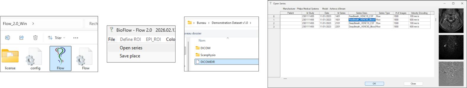
Flow 2.0 is implemented in the Interactive Data Language (IDL) and distributed as a compiled standalone executable. The software does not require a separate IDL license and can be launched directly without installation.
It is primarily designed for Windows systems and can also be executed in macOS environments. On macOS, the IDL Virtual Machine is required to run the .sav file. An X11 environment (e.g., XQuartz) may be required for proper graphical display.
Flow 2.0 requires standard DICOM data organized with a DICOMDIR file.
To load data: Go to File → Open Series; Select the DICOMDIR file; Choose the target RT-PC sequence (the second one).
🧩 Step 2 — Define ROI Location (FOV Centering)
Before segmentation, define the spatial location of the analysis region.
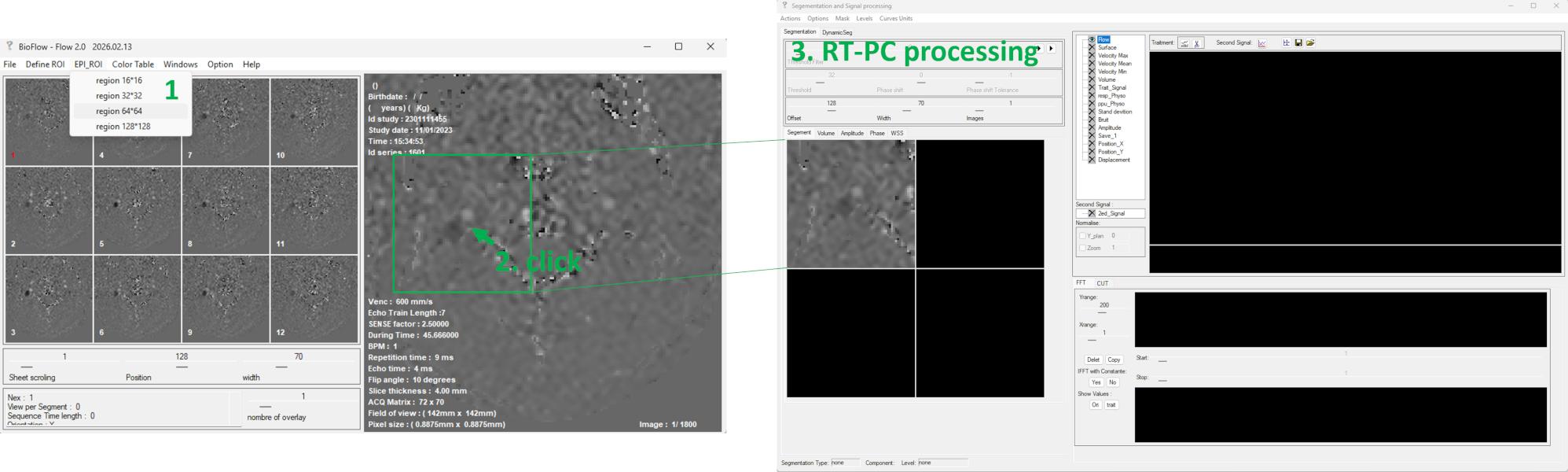
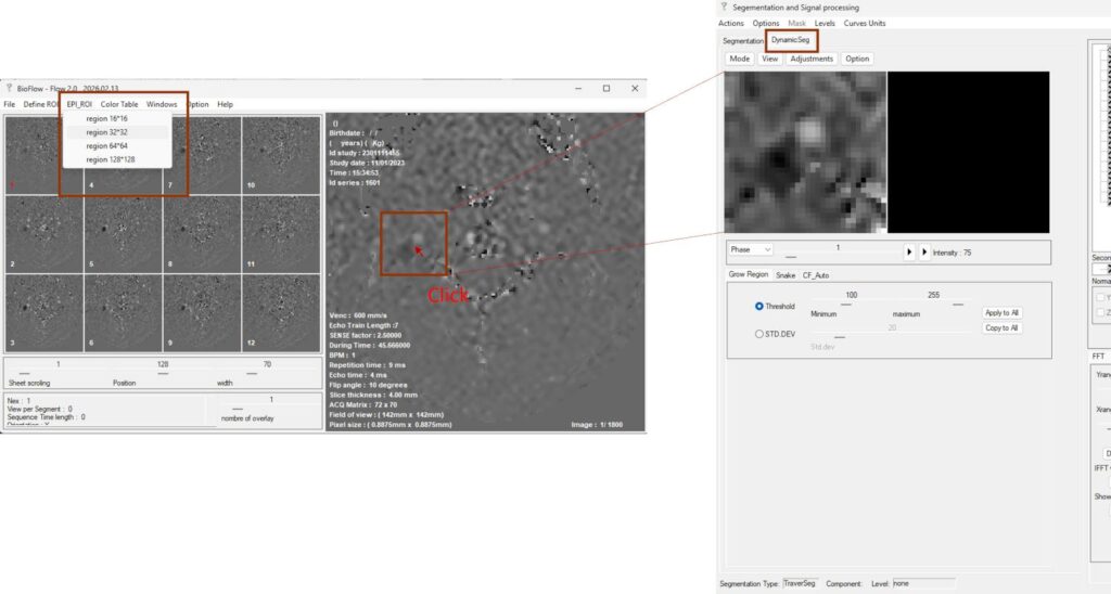
Select an initial field of view EPI_ROI → FOV (e.g., 32 × 32) to launch the RT-PC processing interface; in the main image window, click on the target vessel (e.g., right internal carotid artery, ICA_R).
🧩 Step 3 — Automatic Segmentation
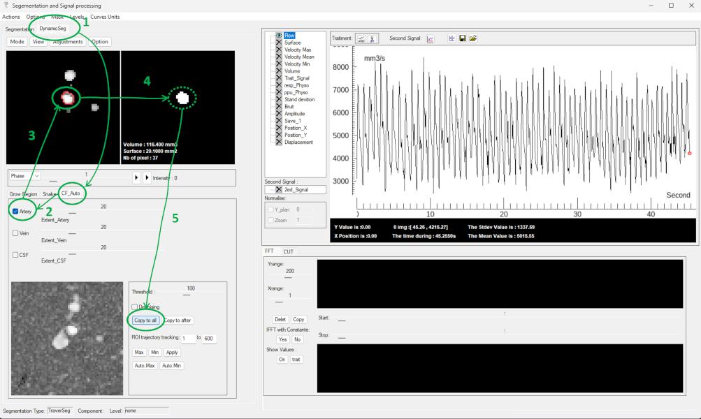
Navigate to: DynamicSeg → CF_auto → Artery, the software automatically detects arterial structures in the left panel.
Select the target vessel from the detected structures → The corresponding ROI is automatically transferred to the right panel → Optional: manually refine the ROI if needed → Click Copy to all to propagate the ROI across all frames.
🧩 Step 4 — De-aliasing (Optional) and Background Phase Correction
Return to the original image display: Adjustments → Original.
Inspect the sequence using the slider or playback. If velocity aliasing is present, apply: Options → Anti-aliasing → e.g. 30%.
Then perform background phase correction (mandatory step): Options → Noise Area Selection → Auto_Definir, this step automatically identifies adjacent static tissue to estimate and correct the phase offset.
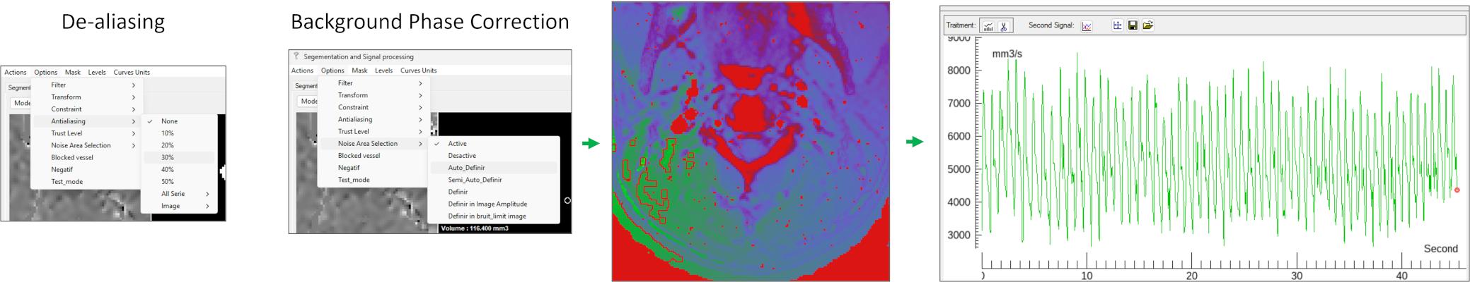
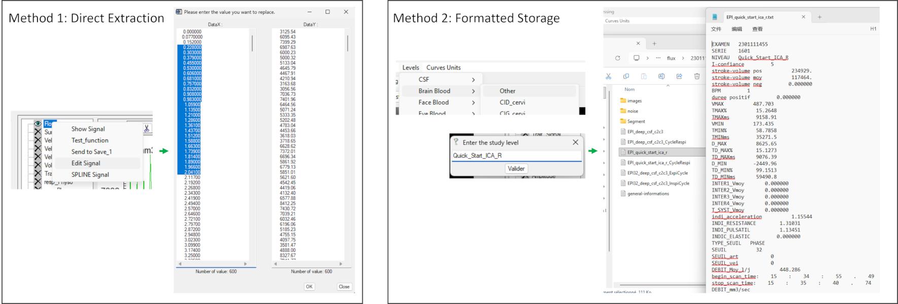
🧩 Step 5 — Visualization and Data Extraction
The processed flow signals are displayed in the signal visualization panel.
You can: Inspect the flow waveform; Interact with the signal for detailed analysis.
To export data: Right-click on the signal you want to view→ Edit Signal to access raw values; Or use Levels to assign labels and export structured results.
1. Introduction
Flow 2.0 is a quantitative post-processing platform for phase-contrast MRI, with dedicated support for real-time acquisitions (RT-PC).
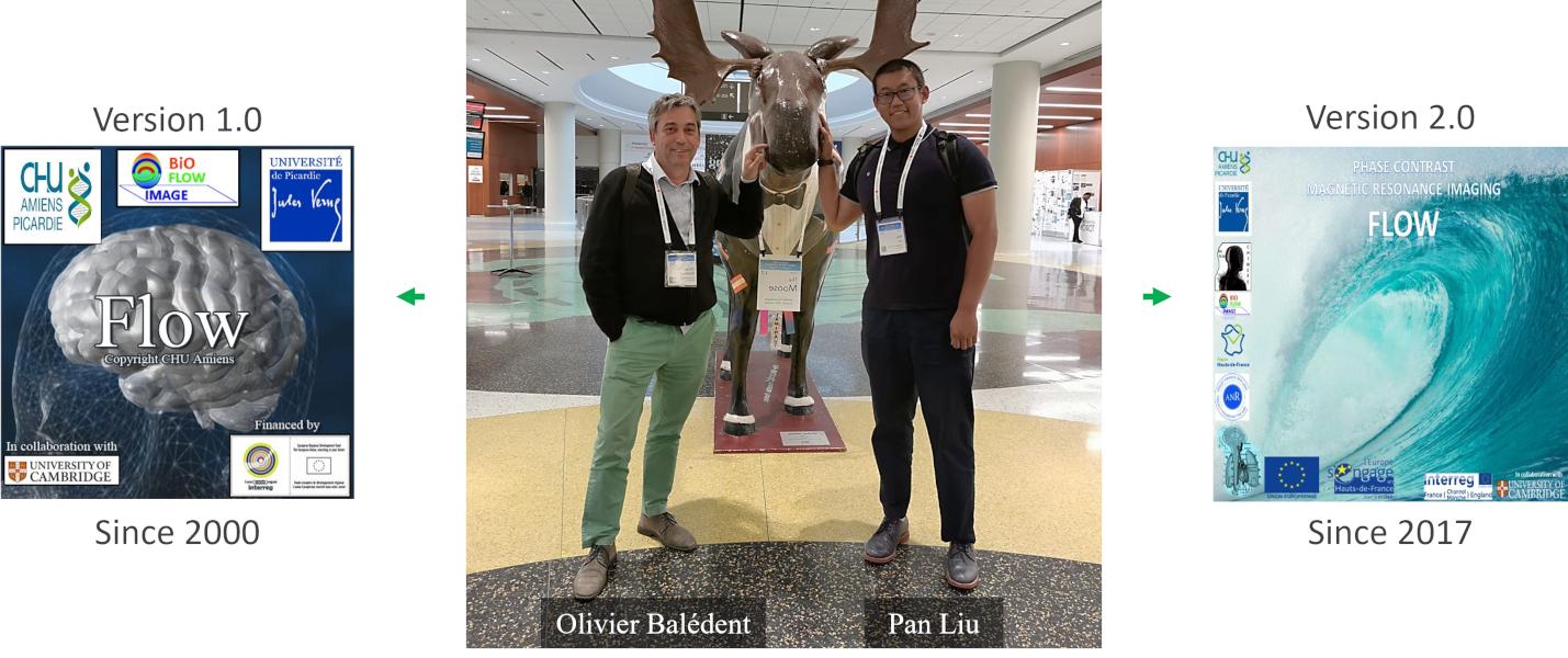
The original framework ( Flow 1.0) was developed in 2000 by Olivier Balédent for cine phase-contrast MRI (CINE-PC), integrating data reading, image segmentation, and quantitative analysis within a unified workflow.
Since 2017, his PhD student – Pan Liu has developed and continuously maintained a new generation of the platform specifically designed for RT-PC, addressing the increased data volume, reduced signal-to-noise ratio, and the need for multi-frequency analysis inherent to RT-PC acquisitions.
Flow 2.0 is currently used in multiple research laboratories and hospital centers for both scientific and clinical-oriented investigations.
RT-PC post-processing typically involves multiple independent steps, including segmentation, background phase correction, and signal analysis, often performed across different tools. Flow 2.0 consolidates these operations into a one-stop framework, enabling highly automated, interactive, and standardized analysis within a single platform.
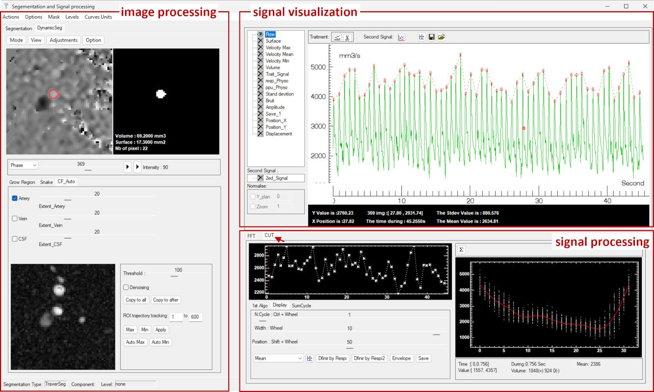
The software is organized around three core modules: image processing, signal visualization, and signal processing, which operate in a tightly integrated workflow. In addition, a dedicated respiratory modulation module enables phase-resolved quantification of physiological influences.
From data import to final quantitative outputs, the entire workflow can be performed within a continuous and reproducible processing pipeline.
This documentation describes the standard workflow and guides users through each step of RT-PC data analysis.
2. Standard Workflow
The analysis follows a continuous pipeline from data import to quantitative output, ensuring consistent and reproducible processing of real-time phase-contrast MRI (RT-PC) data.
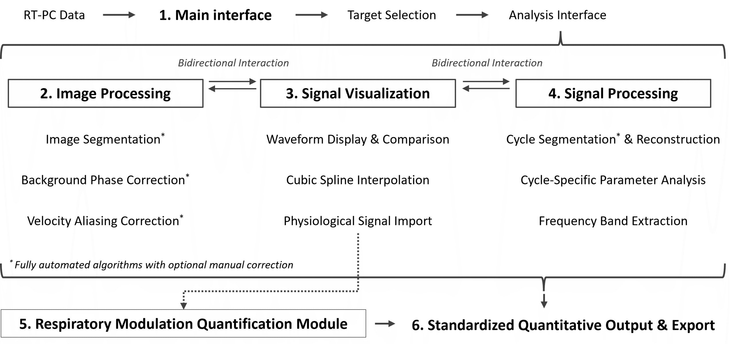
Step 1 — Data Import (Main interface)
RT-PC datasets are loaded from standard DICOM structures.
The target acquisition is selected before entering the main analysis interface.
Step 2 — Image Processing Module
The region of interest (ROI) is defined across the full time series.
Background phase offsets and potential velocity aliasing are corrected to ensure physically consistent measurements.
Step 3 — Signal Visualization Module
Quantitative signals are extracted from the selected ROI and displayed as time-series waveforms.
Waveform navigation is synchronized with image frames to allow direct verification of measurements.
Step 4 — Signal Processing Module
Periodic structures are identified and segmented.
Cycle-based reconstruction and parameter extraction are performed to characterize flow dynamics.
Step 5 — Respiratory Modulation Module
When physiological reference signals are available, phase-resolved analysis can be performed to evaluate modulation effects across respiratory or other periodic inputs.
Step 6 — Data Export and Standardization
Time-series signals and derived quantitative parameters are exported in a standardized format for downstream analysis and reproducibility.
3. Data Import
Demonstration
Video 2. A quick overview of data import and main interface navigation
3.1 Data Import
Software Launch
The software is distributed as a compiled executable and can be launched directly without installation.
On Windows systems, the application can be started by running the executable file.
On macOS systems, the IDL runtime environment is required. After installation, the software can be launched by running the provided flow.sav file.
Save Path Configuration
Before data processing, a default save location can be defined: File → Save place
By default, results are stored in: ...\Flow_2.0_Win\IDL87\flux
Data Import
RT-PC datasets are loaded via: File → Open series
The corresponding DICOMDIR file should be selected. (Only standard DICOM storage formats are supported. Enhanced DICOM format is currently supported for Phillips systems only.)
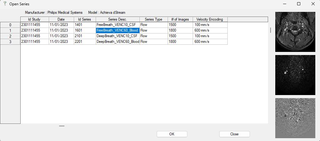
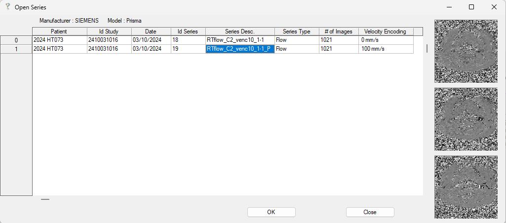
After loading, all available series are displayed in a structured list, including patient name, study ID, acquisition time, series ID, series description, sequence type (e.g., flow for phase-contrast data), number of images, and velocity encoding (VENC).
Selecting the appropriate series completes the data import step.
3.2 Main Interface
Overview
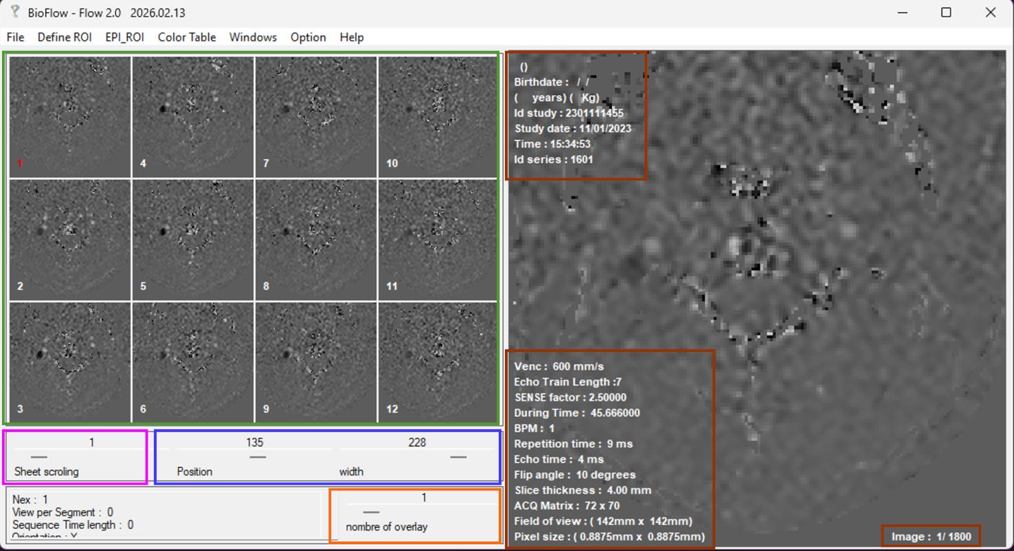
After loading a dataset, the main interface provides synchronized visualization of image data and acquisition parameters.
- The upper-left panel displays a grid of 16 thumbnails across the time series
- The main display panel shows the selected frame with associated sequence information
Several controls are available for navigation and visualization:
- A slider to scroll through time frames
- Two sliders for contrast adjustment (gray-level center and width). Contrast can also be adjusted interactively by dragging the middle mouse button within the main display.
- A slider to combine multiple frames, with the number of overlaid images indicated in the main display
Common Functions
Several utility functions are frequently used during data inspection:
- Option → Information → Deactivate; Hides sequence and patient information (useful for screenshots or anonymization)
- File → Save image as / Save series as; Exports the current frame or the full series to a selected directory
(Avoid saving directly to the desktop for stability reasons) - Option → Window_size → Adaptive_size; Enables interface scaling for smaller screens
- Option → Venc → Set_custom_Venc; Allows manual correction of VENC when not properly detected. The original value can be restored if needed
4. Image Processing Module
Demonstration
Video 3. A quick overview of data import and main interface navigation
4.1 Initialization and FOV Selection
The analysis is initiated from the main interface by selecting an appropriate field of view (FOV) using:
EPI_ROI → 32 × 32 (or other sizes depending on the target structure).
In this example, a 32 × 32 pixel FOV is selected for the internal carotid artery. The RT-PC processing interface is then activated.
The FOV center is defined by clicking directly on the target structure in the main display window, after which the corresponding data are displayed in the RT-PC analysis interface.
Dynamic segmentation is performed in the DynamicSeg panel, where each frame has its own ROI. The Segmentation panel is dedicated to CINE-PC post-processing (see Flow 1.0 documentation).
4.2 Overview
This module performs ROI segmentation (section 4.4) and enables the extraction of flow-related parameters from RT-PC data. It also includes velocity aliasing correction (section 4.6) and background phase correction (section 4.7) to ensure accurate measurements.
Additional image processing and visualization tools (section 4.3) are provided to support segmentation and data inspection.
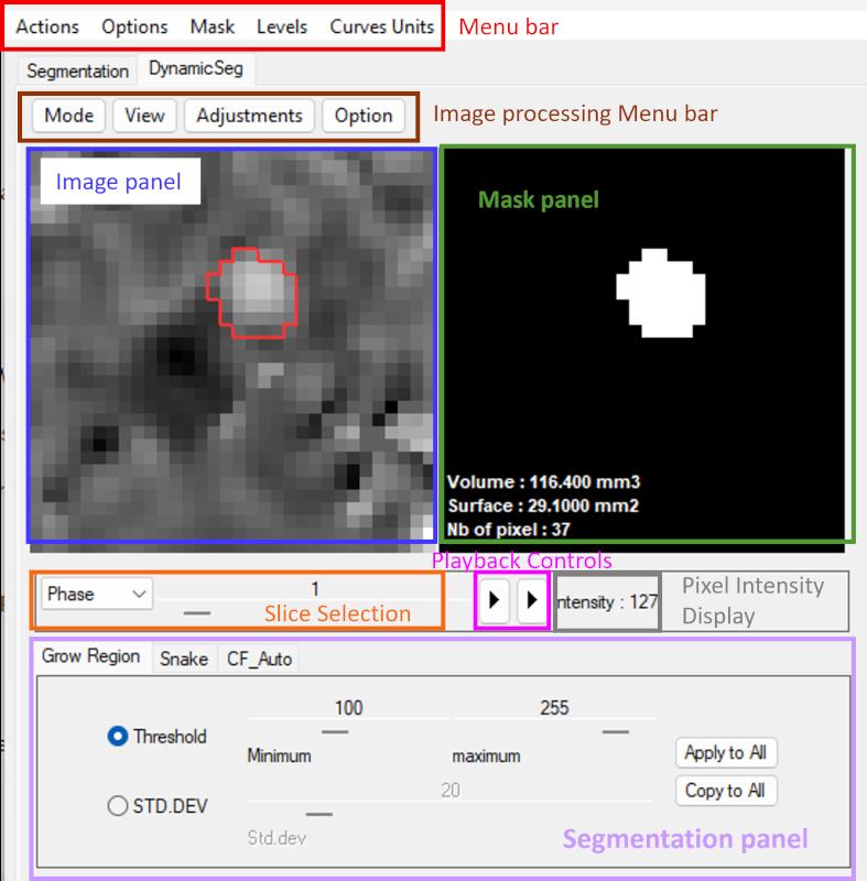
The interface is organized into several functional regions:
- The image processing menu bar provides access to processing and visualization tools.
- The image display panel shows the current frame (Allow the mouse wheel to scroll through images).
- The mask panel displays the segmented ROI. Includes manual ROI refinement and basic morphological operations (see Section 4.5).
- The slice selection allows browsing through frames.
- The playback controls enable dynamic visualization of the sequence.
- The pixel intensity display provides the value of the current pixel in image panel.
- The segmentation panel provides access to the three ROI definition methods.
4.3 Image Preprocessing Tools
Several basic image processing tools are available to support segmentation and visualization.
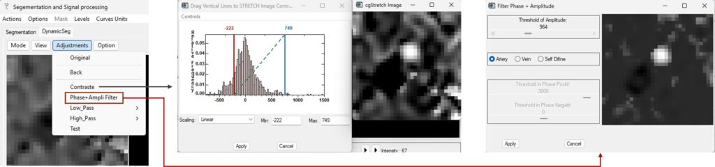
Two commonly used functions are highlighted below:
- Adjustments → Contrast: Adjusts the contrast of the current image (magnitude or phase). The display range can be interactively defined by adjusting the red and blue bounds.
- Adjustments → Phase–Amplitude Filter: Performs noise reduction by combining magnitude and phase information. The filtering mode (artery or vein) can be selected, and the threshold can be adjusted accordingly. This operation can be applied multiple times if needed.
Additional utility functions include:
- Adjustments → Back: Restores the previous processed image.
- Adjustments → Original: Reloads the original image.
- Option → Load_ROI: Loads previously saved ROI data from the corresponding segment folder. Previously defined ROI and background correction settings are restored automatically, enabling consistent re-analysis.
Other available tools include low-pass filtering, high-pass filtering, and 3D visualization (View → 3D Visualization), which can be used for specific visualization or exploratory purposes.
4.4 Three Segmentation Strategies
This module provides three segmentation approaches, allowing selection of the most appropriate method depending on the target structure and its motion characteristics.
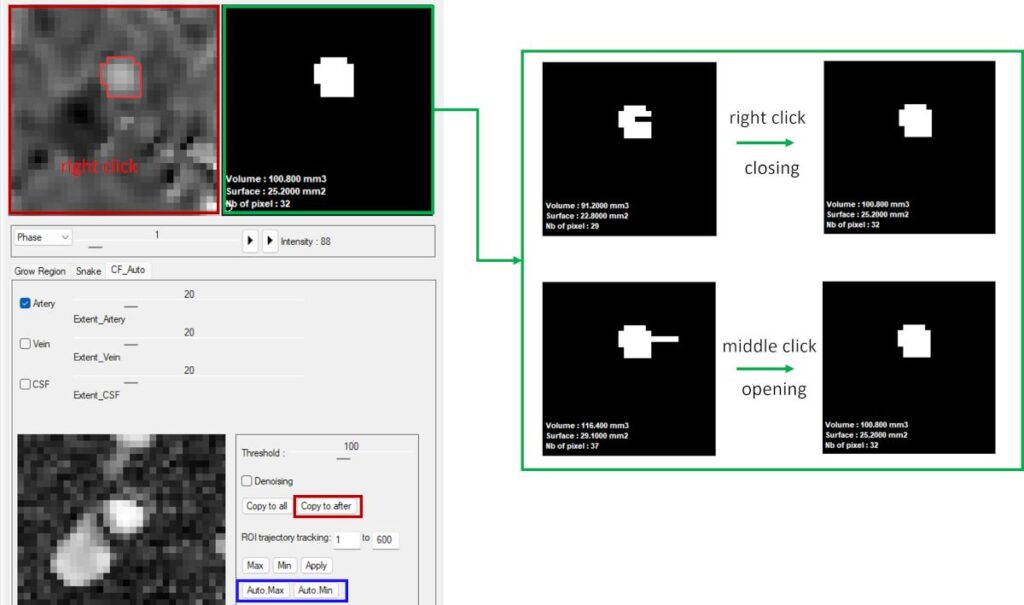
4.4.1 CF_auto (Characteristic Frequency Automatic Segmentation)
CF_auto is an automatic segmentation method specifically developed for neurofluid applications.
It identifies pulsatile structures by analyzing the contribution of cardiac frequency components, enabling extraction of cerebral arteries, veins, and CSF.
This approach provides a simple and efficient solution for neurovascular segmentation and is the recommended default method for RT-PC data.
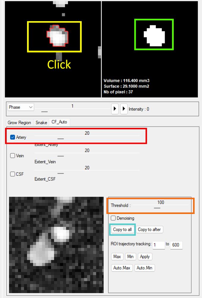
Segmentation is performed by selecting the target type (artery, vein, or CSF), after which candidate ROIs are automatically detected and displayed in the image panel.
Threshold-based refinement is available to adjust the ROI boundaries.
The selected ROI can then be transferred to the mask panel, and multiple ROIs can be combined if needed.
Click “Copy to all” to copy the ROI to all frames.
An example is shown in the video, where arterial, venous, and CSF structures are segmented from the same slice using datasets with different VENC settings (e.g., 60/10 cm/s).
Video 4. A quick overview CF_Auto Segmentation.
CF_auto generates a fixed ROI across frames and is therefore best suited for structures with limited deformation, such as cerebral vessels and CSF.
For periodic motion or small displacements, additional correction can be applied using the ROI adjustment tools (see Section 4.6).
4.4.2 Snake Segmentation (Active Contour-Based Dynamic Segmentation)
This method is designed for structures with significant deformation or displacement, such as large vessels (e.g., coronary arteries or portal veins).
It is based on an active contour (snake) model, where the ROI evolves iteratively by balancing curvature, smoothness (viscosity), gradient strength, and iteration number. The resulting contour is propagated frame-by-frame, using the final contour of each frame as the initialization for the next, enabling fully automatic dynamic segmentation across the time series.
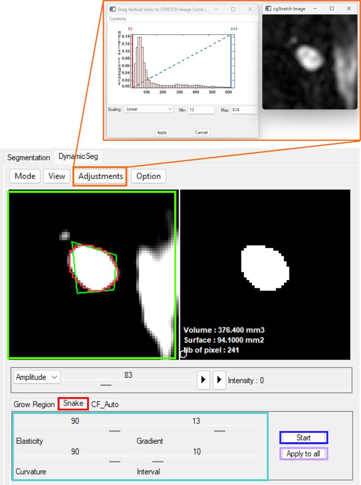
In practice, segmentation is typically performed on magnitude images. After selecting the Snake panel, contrast can be enhanced to improve vessel visibility.
An initial contour (Left mouse button) is then defined in the image panel, followed by adjustment of the main parameters (curvature, viscosity, gradient strength, and iteration settings).
The segmentation result can be tested on a single frame before applying the configuration to all frames. Once validated, dynamic segmentation is performed automatically across the sequence.
Manual refinement remains available for specific frames when local corrections are required.
An example is shown in the video (first part), where dynamic segmentation of the portal vein is performed using the snake method. A comparison with region-growing segmentation is also provided.
Video 5. Snake Segmentation and Grow Region Segmentation in Portal Vein
Snake segmentation is less effective for very small structures (typically fewer than ~16 pixels) and may become computationally expensive when a large number of iterations is required. For structures with strong contrast and sufficient pixel coverage, larger parameter values can be used to reduce the number of iterations.
4.4.3 Region-Growing Segmentation
This method is designed for the same targets as snake segmentation, namely structures with significant deformation or motion.
It is based on a region-growing strategy, where the centroid of the ROI in each frame is used as the seed for the next frame, enabling dynamic propagation across the time series.
An example is shown in the second part of Video 5, where dynamic segmentation of the portal vein is performed using this method.
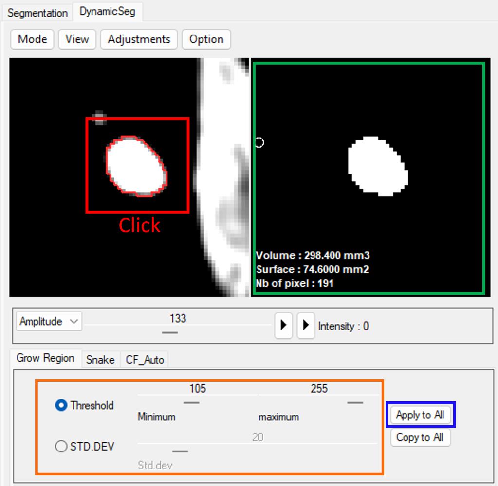
Segmentation is initialized by selecting a seed point in the image panel.
The ROI is then defined based on an intensity threshold, which can be specified either directly or relative to the local signal variation (standard deviation).
The resulting region is displayed in the mask panel.
Once the parameters are set, segmentation can be applied to all frames for automatic propagation.
Compared with Snake methods, Region-growing is generally faster and efficient for structures with high contrast and well-defined boundaries. However, it is more sensitive to leakage when boundaries are weak or noisy. In such cases, additional refinement or alternative methods may be required.
This method can also be used for single-frame ROI adjustment, providing a convenient tool for local corrections.
4.5 ROI Adjustment
After automatic segmentation, ROI inaccuracies may arise from three main situations: local segmentation errors in individual frames, global displacement during acquisition, and small periodic motion (e.g., cardiac or respiratory-induced shifts). Corresponding correction strategies are provided for each case.
Manual ROI Refinement
Local errors in individual frames can be corrected manually. The signal visualization module can be used to identify abnormal frames, for example through surface waveform.
After locating the target frame, the ROI can be modified directly in the mask panel.
Using the left mouse button, pixels can be added to or removed from the ROI depending on the state of the clicked pixel. Clicking on a pixel inside the ROI activates removal, whereas clicking outside the ROI activates addition.
The brush diameter can be adjusted with the mouse wheel.
Two basic morphological operations are also available for rapid correction: right click performs closing, and middle click performs opening. These operations help refine ROI shape and improve mask continuity.
ROI Translation and Propagation
Global displacement, such as subject motion or swallowing, can be corrected by translating the ROI.
After selecting the image panel (by right click), the ROI can be shifted using the keyboard (arrow keys or W/A/S/D).
This allows direct alignment of the ROI with the target structure in the current frame.
Once the ROI position is corrected, it can be propagated to subsequent frames using the Copy to after function (in the CF_auto panel), enabling efficient correction across the remaining time series.
Automatic ROI Adjustment
For small periodic displacements, such as those induced by cardiac or respiratory motion, automatic ROI adjustment can be applied.
This function is available in the CF_auto panel via Auto.Max or Auto.Min.
For each frame, the ROI is shifted within a local neighborhood (pixel-level search), and the position that maximizes or minimizes the total signal intensity is selected.
The operation can be applied iteratively to improve temporal consistency of the ROI across frames. However, care should be taken in low-contrast conditions, where incorrect alignment or drift may occur.
4.6 Velocity Aliasing Correction
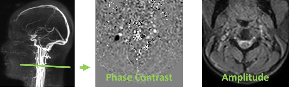
Velocity aliasing occurs when the measured velocity exceeds the encoding range (VENC), resulting in non-physical intensity changes.
For example, velocities between VENC and 2×VENC may appear with inverted contrast (e.g., bright arterial pixels becoming dark), as illustrated in the figure.
Aliasing can be rapidly detected using the Velocity Max signal in the visualization module, which displays the maximum absolute velocity within the ROI.
Abrupt or inconsistent values indicate the presence of aliasing and allow direct localization of the affected frame.
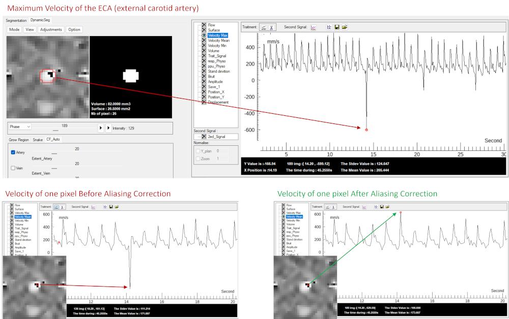
Correction can be applied via:
Options → Antialiasing → All Series → Positive
In this mode, all pixels within the ROI are assumed to follow a positive flow direction.
Negative values are identified as aliased and corrected accordingly, restoring physically consistent velocity measurements.
As shown in the figure, the corrected signal recovers the expected velocity profile after aliasing removal.
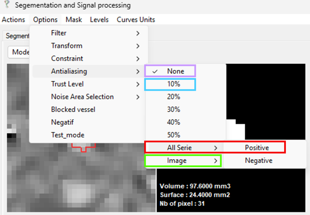
Additional options are available for more flexible correction:
- Options → Antialiasing → Image → Positive / Negative
Applies aliasing correction to the current frame only - Options → Antialiasing → 10%
Corrects pixels exceeding the VENC threshold within a limited range (±10%), with direction determined by the mean ROI velocity. This function is particularly suitable for correcting CSF flow with bidirectional velocity changes. - Options → Antialiasing → None
Disables aliasing correction
4.7 Background Phase Correction
In phase-contrast MRI, non-zero velocity offsets may appear in static tissue due to gradient imperfections, eddy currents, or magnetic field inhomogeneities. These offsets can affect the accuracy of flow quantification.
This module provides background phase correction by selecting static tissue regions surrounding the target vessel or CSF. The mean velocity of this region is used to redefine the zero-velocity baseline on a frame-by-frame basis, removing systematic offsets.
Lower VENC values are more susceptible to background phase offsets. Here, CSF at the C2–C3 level with VENC = 10 cm/s is used as an example.
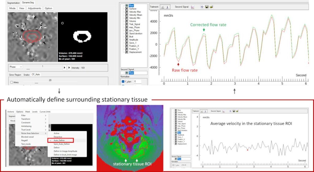
Automatic Background Phase Correction
Options → Noise Area selection → Auto_Definir
An automatic method is applied by default to identify static tissue around the ROI.
This approach requires no prior knowledge or user intervention and is suitable for most cases.
The selected static region is displayed in the interface, allowing visual verification.
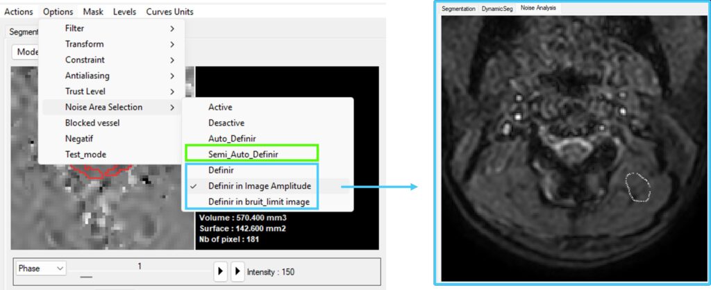
Semi-Automatic Background Phase Correction
Options → Noise Area selection → Semi_Auto_Definir
This method builds upon the automatic selection but allows adjustment of the region size used for background estimation.
It is useful in more complex situations where refinement of the static region is required.
Manual Background Phase Correction
Options → Noise Area selection → Definir / Definir in amplitude / Definir in bruit_limit_image
Static tissue can be manually defined on different image types.
This approach requires prior knowledge and is typically used when automatic methods are not sufficient.
A closed ROI is drawn using the left mouse button, and the selection is confirmed with a right click.
Correction Output and Visualization
After background phase correction, the flow signal displayed in the visualization module changes from black to green, indicating that baseline correction has been applied.
The corrected signal reflects the true flow dynamics with the velocity baseline properly centered around zero.
5. Signal Visualization Module
Demonstration
Video 3. A quick overview of data import and main interface navigation
5.1 Overview
This module serves as a bridge between image processing and signal processing, enabling real-time interaction between modules for efficient and intuitive analysis.
It allows visualization, comparison, and manipulation of multiple signals derived from the ROI.
Signals can be translated, scaled, and inspected directly within the main display, facilitating interactive exploration of flow dynamics.
In addition, the module supports dual-signal comparison and integration of external physiological signals.
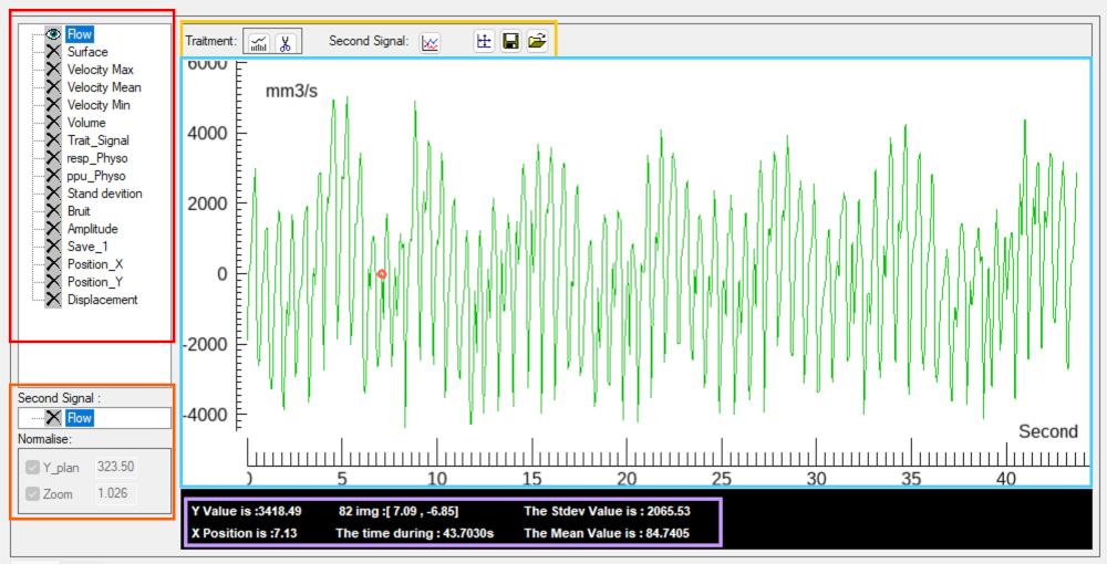
The interface is organized into several functional components:
- Signal list panel
Displays all available signals derived from the ROI, allowing selection and activation of individual parameters. - Dual-signal comparison panel
Enables simultaneous visualization and comparison of two signals with independent scaling and alignment options. - Function panel
Provides access to signal processing tools, including time-domain processing, frequency-domain analysis, display reset, and physiological signal loading. - Main visualization panel
Displays the selected signal(s) as time-series waveforms for inspection and comparison. - Information panel
Displays quantitative information in three sections:
(1) the current cursor position (X, Y),
(2) the corresponding image frame and signal value at the tracked point (red marker),
(3) the mean value and standard deviation of the selected signal.
5.2 Signal List Panel
The signal list stores all available signals and is automatically updated following any processing step, including ROI modification, background phase correction, velocity aliasing correction, physiological signal loading, and signal processing operations.
The following signal types are available:
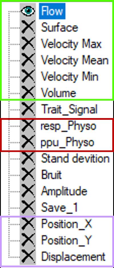
Flow: Volumetric flow rate within the ROI (area × mean velocity)
Surface: ROI area over time, used for dynamic deformation
Velocity Max/Min: Maximum and minimum velocity within the ROI
Velocity Mean: Mean velocity within the ROI
Trait_Signal: Post-processed signal (frequency-domain extraction)
resp_Physio: Respiratory signal (chest belt)
ppu_Physio: Peripheral pulse signal
Standard Deviation: Velocity standard deviation within the ROI
Bruit: Mean velocity of static tissue (after background correction)
Amplitude: Mean magnitude intensity within the ROI
Save_1: User-defined stored signal
Position_X/Y: ROI centroid coordinates
Displacement: ROI centroid displacement relative to the first frame
5.3 Signal Display and functions
Signals can be selected using the left mouse button, and the selected signal is displayed in the main visualization panel.
Active signals are indicated by an eye icon, while inactive signals are marked with a cross icon.
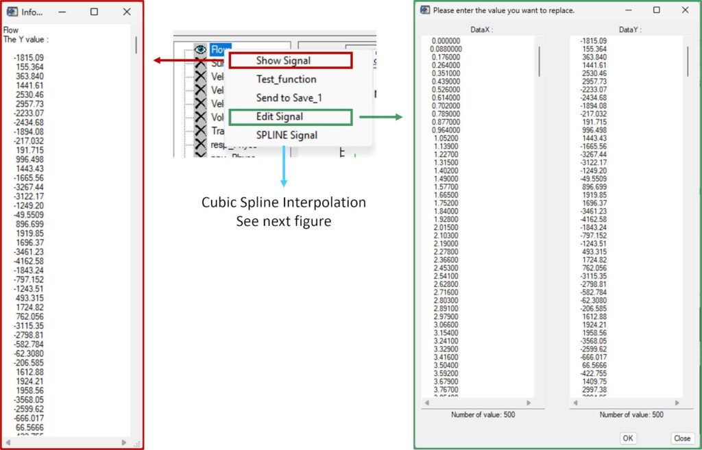
Right-clicking a signal opens a context menu with the following functions:
- Show_Signal: Displays the signal as a copyable text list (Y values over time)
- Edit_Signal: Opens an editable table of X and Y values for manual modification
- SPLINE_Signal: Applies cubic spline interpolation to the selected signal
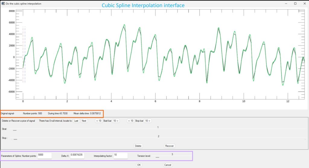
The spline interface displays the original signal together with the interpolated result.
The top information panel displays the original signal information.
Interpolation parameters are defined in the lower panel (number of points, Δt, interpolation factor, and tension level). The first three are interdependent, and modifying any one automatically updates the others.
5.4 Physiological Signal Import
…
5.5 Dual-Signal Comparison
…
5.6 Main Display Panel
…
5.7 Interaction with Image and Signal Processing
…
This user manual is currently being finalized and is expected to be completed in June 2026. If you have any questions regarding specific procedures, please feel free to contact Pan Liu at any time; your questions will be addressed promptly.